Detailed Explanation of Neural Network Layers and Propagation

let’s dive deeper into the details of neural networks, focusing on their structure, the role of different layers, and how they process inputs. We’ll use a simple example of an image classification task to illustrate these concepts.1. Input LayerThe input layer is the first layer of a neural network and receives the raw input data. Each neuron in this layer represents one feature of the input data.Example:
For an image classification task, consider a grayscale image of size 28×28 pixels. The input layer will have 784 neurons (since 28*28 = 784), each representing one pixel value.2. Hidden Layers

Hidden layers are the intermediate layers between the input and output layers. They perform various transformations on the input data to extract features and patterns. Each neuron in a hidden layer takes inputs from the previous layer, applies a weighted sum, and passes the result through an activation function.

Example: Let’s consider a neural network with two hidden layers:

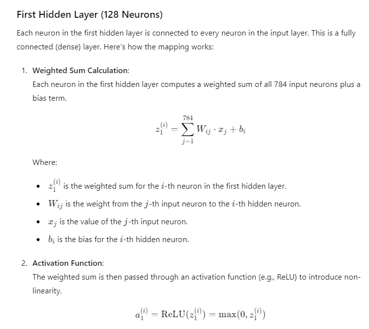
• First hidden layer: 128 neurons
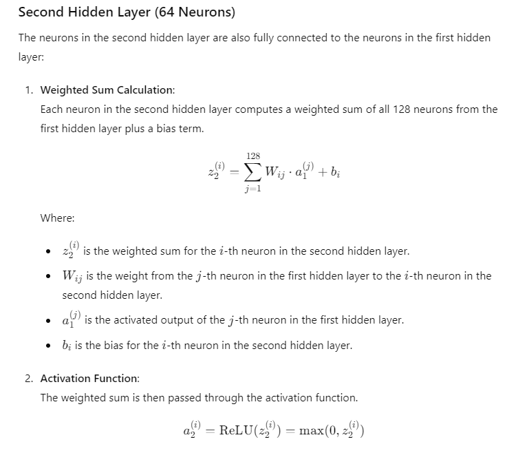
• Second hidden layer: 64 neurons

3. Output Layer

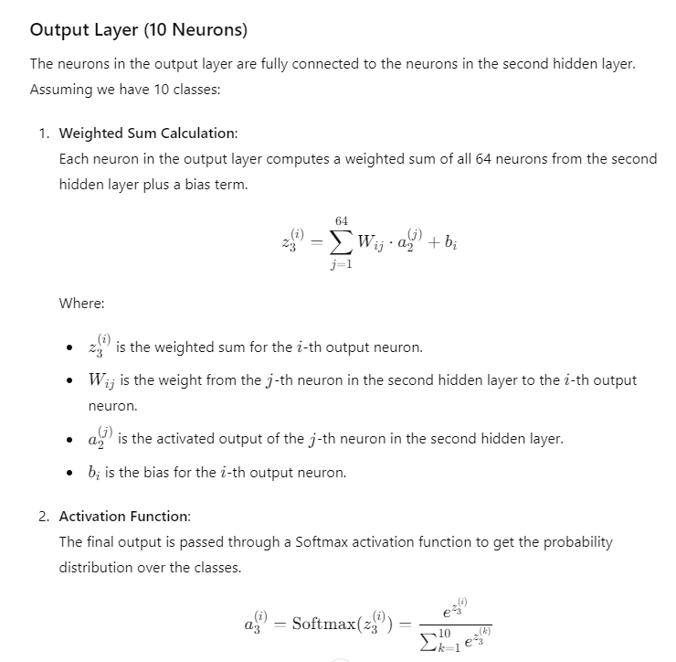
The output layer produces the final prediction. The number of neurons in this layer corresponds to the number of possible classes in the classification task.

Example: For an image classification task with 10 possible classes (e.g., digits 0-9), the output layer will have 10 neurons. The activation function used in this layer is typically Softmax, which converts the raw scores into probabilities.

Neural Network Architecture Example

Here’s a simple example of a neural network for classifying 28×28 grayscale images into 10 classes:

1. Input Layer: 784 neurons (one for each pixel)
2. First Hidden Layer: 128 neurons, ReLU activation
3. Second Hidden Layer: 64 neurons, ReLU activation
4. Output Layer: 10 neurons, Softmax activation

Detailed Steps

1. Initialization:
   • Initialize weights and biases for all layers.
   • Typically, weights are initialized with small random values, and biases are initialized to zero or small constants.
2. Forward Propagation:

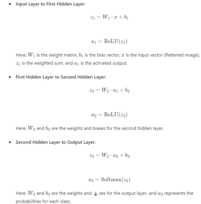
Let’s clarify the mapping process in the context of a neural network, focusing on how data flows from one layer to another.

Input Layer (784 Neurons)

For an image classification task using a 28×28 pixel grayscale image, the input layer has 784 neurons because: 28×28=78428 \times 28 = 78428×28=784

Weights Matrix (W)

1. What is W?
   • WWW is a weights matrix that connects neurons from one layer to the next. Each element in this matrix represents the strength of the connection between two neurons.
2. Initialization:
   • The weights matrix is typically initialized with small random values. This randomness helps to break symmetry and allows the neural network to learn different features.
3. Updates During Training:
   • During training, the values in the weights matrix are updated in each iteration (or epoch) using an optimization algorithm (like Stochastic Gradient Descent, Adam, etc.). This process is guided by the gradients computed during backpropagation, with the aim of minimizing the loss function.